Predicting the London Boredom Index

Amidst the ongoing Covid-19 pandemic, the UK government adopted various measures to contain infections locally. Compliance with these restrictions may be affected by citizens' levels of frustration and boredom, requiring accurate monitoring of public sentiment and continual calibration of policy stringency as the situation unfolds.

I proposed using Covid-19 infection case numbers in London, indices measuring the stringency of government policy and the level of public transportation usage in the London metropolitan area to forecast the percentage of Londoners experiencing boredom. I subsequently created a Python notebook in order to compare and contrast two time series approaches.

Data Collection

First I aggregated six datasets into a single time series covering the period between the 2^nd of March and the 21^st of September, 2020 with a daily frequency:

New cases and cumulative total cases of Covid-19 infections in London (provided by Public Health England);
The policy stringency index for the United Kingdom, a percentage measuring the stringency of government pandemic-control measures (provided by the developers of the Oxford Coronavirus Government Response Tracker);
The Citymapper mobility index for London, a ratio comparing the general number of planned journeys with a baseline period between the 6^th of January and the 2^nd of February, 2020 (provided by the developers of the transit planning app Citymapper);
Community mobility indices for workplaces and residential locations, two ratios comparing the number of planned journeys for the respective purposes of employment and domestic activity, with a baseline period between the 3^rd of January and the 6^th of February, 2020 (provided by Google);
The Tube ridership index, a ratio comparing the number of daily Tube journeys with the equivalent day in 2019 (provided by Transport for London);
The boredom index, the percentage of surveyed respondents who expressed boredom as their main mood for a given week, with daily values interpolated as constant between survey dates (provided by YouGov).

The first dataset measures the prevalence of infection within the London population, while the second dataset measures the extent of governmental responses. With both of these information sources we may distinguish between different phases in the pandemic (e.g. there will be a lag between increased stringency and new case numbers). The latter three datasets measure London residents' movements using public transportation and are a proxy for human levels of activity.

Problem Formulation

Given all but the last seven days of input data, the prediction target is the daily boredom index for the last week.

Two potentially suitable models to predict the daily boredom index include an auto-regressive moving-average process with exogenous inputs (ARMAX) or a recurrent neural network architecture such as the gated recurrent unit (GRU).

Model Development: ARMAX

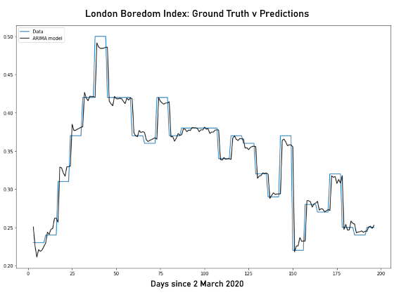
An ARMAX model involves a linear combination of previous target estimates (of public boredom), external inputs (case numbers, policy stringency, usage of public transportation), and random noise. I opted to use two auto-regressive terms and three moving-average terms. The graph below plots the predictions of the model on the training set after fitting the parameters using maximum likelihood estimation.

Model Development: GRU

If the boredom index time series does not exhibit stationarity (perhaps due to shocks caused by suddenly increased policy stringency), it may not be appropriate to use the ARMAX model. The GRU model computes a non-linear combination of the inputs over time.

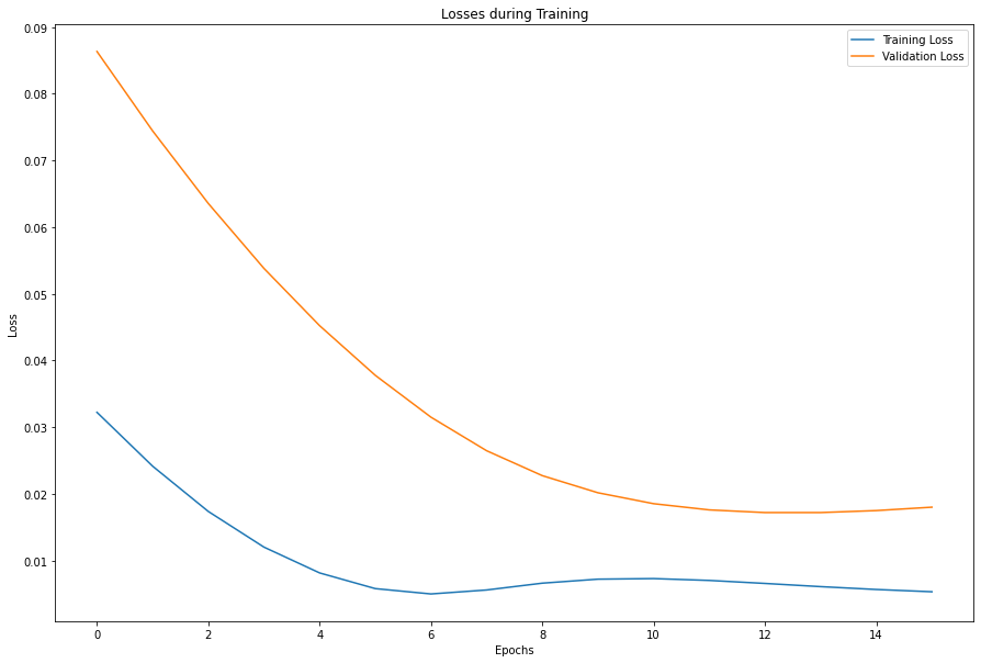
After brief testing of hyperparameters I chose to use a two-layer GRU, taking as input all data except the boredom index. The hidden output of the final layer is of dimension 7 and is fed to a linear layer. Finally, the linear layer's scalar output is passed through a sigmoid function to constrain the output to the range [0,1]. The graph below plots the losses incurred during training, with early stopping when the validation loss increases.

Results

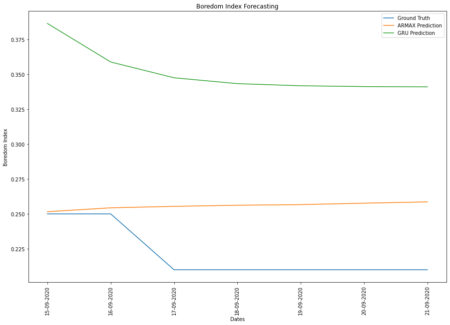
Comparing the predictions of the ARMAX and GRU models for the last seven days of the dataset in the graph below, we can observe that the ARMAX has a much lower root mean square error (3.97×10^-2) than the GRU model (1.32×10^-1).